Tag: machining

  • A brief study on sharpening stones – Part 7 – Schleifjunkies Resinbond Stones (6- 3- 1 µm)

    A brief study on sharpening stones – Part 7 – Schleifjunkies Resinbond Stones (6- 3- 1 µm)

    This is part of a series of blog posts – looking into the appearance and composition of commercially available sharpening stones. If you are interested in the previous episodes:

    Part 1 is about the Fällkniven DC3 , Part 2 is about the DMT mini W7C, Part 3 is about the TSPROF Blitz F1000, Part 4 is about a natural jade stone, Part 5 is about the Venev 5/3 Diamond Resin Stone, Part 6 is about the Edge Pro Matrix Stone (4000 grit).

    If you have some suggestion on what I should look at next, or want to share your super secret DIY stones, I could be persuaded to open the bag of analytical devices… hit me up on Instagram under @marvgro for that.

    Review
    Today’s sharpening Stone is a triplet of stones. These are from a German sharpening shop called “Schleifjunkies”. The stones are advertised under the name “resinbond”, and according to the manufacturer create high gloss and super sharp edges in minutes, not hours. Ok! Let’s take a closer look 🙂

    The stones are well finished on the top surface, with a smooth, green surface. The side is raw and appears to be saw or maybe beam cut? They are actually glued down to the holder with some flexible foam tape, allowing for some flex between stone and aluminium holder:

    Let’s take a look at each stone under the optical microscope.

    Optical micrographs of the SJ Resinbond 6 µm stone. The scale bar is visible in the lower right corner. Instrument: Leica Emspira.

    Quite a bit of colour is visible at higher magnifications. Green, translucent green (typically diamond), black, and some reddish-orange colour. I think this is going to be a very interesting stone to look at under the SEM.

    Optical micrographs of the SJ Resinbond 3 µm stone. The scale bar is visible in the lower right corner. Instrument: Leica Emspira.

    Optical micrographs of the SJ Resinbond 1 µm stone. The scale bar is visible in the lower right corner. Instrument: Leica Emspira.

    The two finer stones show about the same colour – the translucent green particles do shrink in size though, most notably from 6 to 3 µm. I can’t really tell any difference in size on the other particles.

    The stone was cleaned with IPA in an ultrasonic bath, rinsed and then blow-dried with compressed, ultra pure nitrogen gas before getting put into the SEM.

    SEM Micrographs of the SJ resinbond 6 µm stone. Instrument: Zeiss GeminiSEM560.

    The stone is a mix of 3 different, easily identifiable grains. There are larger, above 10 µm grains all across the surface, in a low conecntration. there is a higher concentration of smaller, blocky, fractured grains as well as a notable amount of rounded grains, that have some molten look to them. Between the grains, some areas are binder (matrix / resin) dense, whereas others are dense agglomerations of grains.

    SEM Micrographs of the SJ resinbond 3 µm stone. Instrument: Zeiss GeminiSEM560.

    The 3 micrometre stone shows the wide spread of grains, and also their diverse size:

    There are some 10 µm sized grains, that are very long and narrow, interspersed with some more blocky, rounded grains that I suspect will be the diamond. On the upper left corner, one can make out the molten droplets in fine detail. These are also a bit lighter colour – typically a sign that they consist of a heavier element than the surroundings. I took a quick peak at the 1 micrometre stone, which looked nearly identical to the 3 micrometre one, but didn’t go through the trouble of recording the images, as I prefered to focus on finding out all it’s secrets – especially the 3 different grains that are visible! For this, I did energy dispersive x-ray spectroscopy (EDS) to create elemental composition maps over the SEM picture.

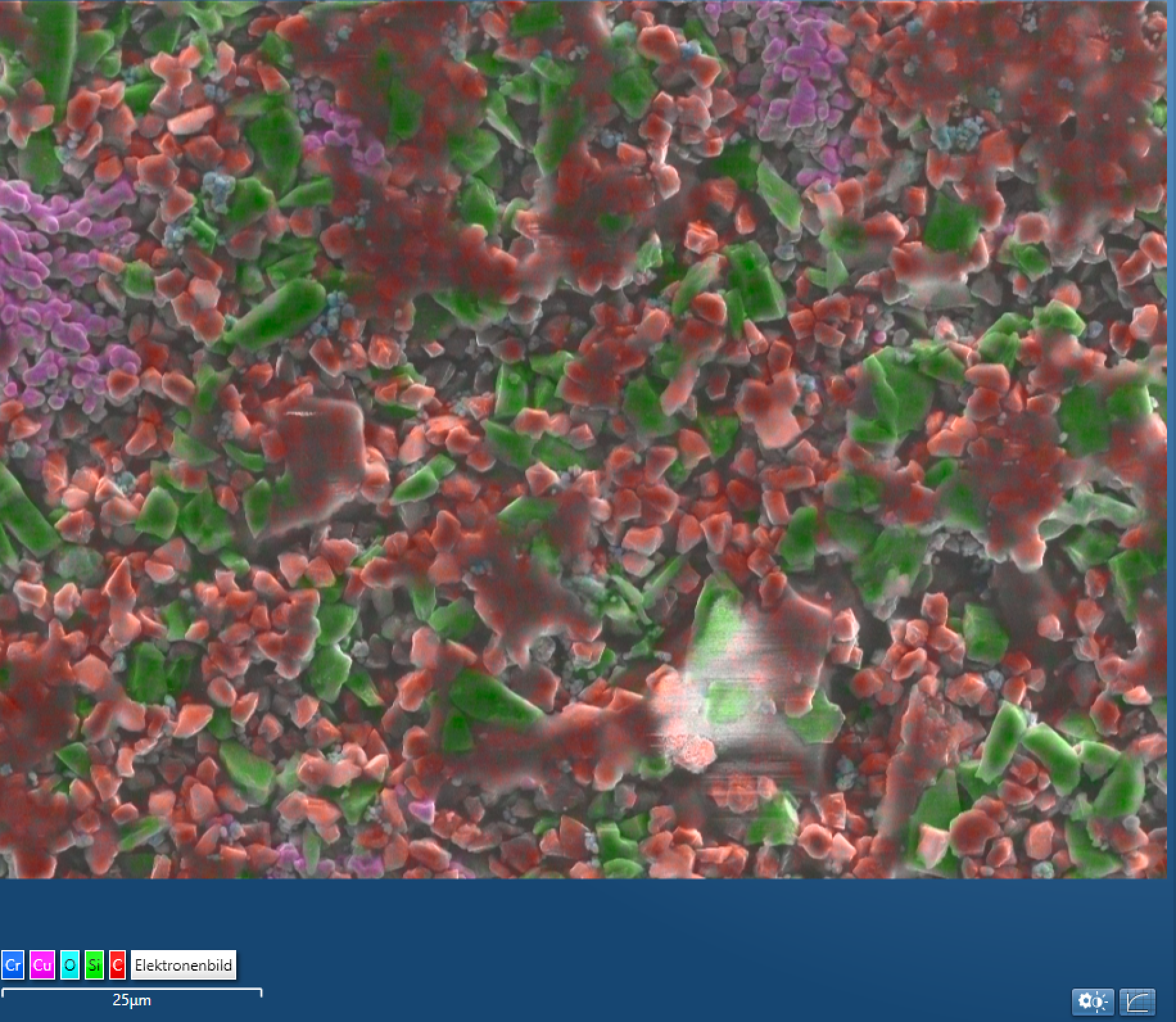
    EDS analysis of the Schleifjunkies 3 micrometre resinbond stone. Instrument: Oxford Ultim Max  ∞ 40mm2 EDS sensor. Note that our EDS sensor doesn’t show elements lighter than boron.

    The EDS analysis brings some clarity to this! Let’s take a closer look at the elemental mapping ,and what we can deduce from this.

    The stone has some large, blocky, molten looking red areas, which are carbon rich. This is the resin used to bond the particles together. The smaller, red grains are also mainly carbon – most definitely the diamond grain. SJ seems to have used a more blocky, smoother grain shape here.

    THe green grains are silicon, but by comparing the carbon intensity map, we can see that they also consist of carbon. This is silicon carbide, at about 3 times the size of the diamond grains. Silicon carbide is quite hard (2400-3000 HV, depending on the type), which is why it is often used as an abrasive on it’s own. The use in resin bond stones is typically to make the bond harder. The purple grains are actually copper – which explains the reddish grain we could make out in the optical microscope pictures. Copper is added to industrial resin grinding wheels to improve heat conductivity, and while this makes a lot of sense at high cutting speeds, and if your abrasive is alumina oxide (corundum) or SiC, diamond has a much better heat conductivity, and it’s the first time I’m seeing this on a diamond grinding bit. Frankly, here it can only be either a cheap filler, or the manufacturer took the same mix they use for AO grinding wheels and just added diamond. Trace amounts of chromium can be detected, as well as some oxygen, matching particles with the silicon map, so I’d suspect that the rare, white-ish particles we have seen in the microscope are SiO2 (quartz) particles.

    Let’s take a look at the surface roughness and appearance.

    3D height map of the 6 µm SJ resinbond stone. Instrument: Bruker Alicona µCMM, 50X objective lens, singe FOV high resolution focus variation scan. Data is leveled and outliers removed (0.25%). 2nd picture: area extract to show the grain.

    The surface, similar to the SEM picture, has large, very smooth sections, where the grain is still covered in a bit of resin, and also irregular, smaller sections with voids and recessed grains. This matches the view from the SEM quite well.

    ISO 25178 parameters of the 6 µm SJ resinbond stone.

    The stone surface roughness (Sq) is very low, with a nice and tight control on the height of the surface bearing material ratio (Sdc). The kurtosis (Sku) is quite high here, a result of the very flat sections in combination with the very steep walls leading down to the voids. This smooth stone will glide quite easily along a blade, while providing little feedback. The pressure applied is spread over a large area, reducing the force acting on every grain.

    3D height map of the 3 µm SJ resinbond stone. Instrument: Bruker Alicona µCMM, 50X objective lens, singe FOV high resolution focus variation scan. Data is leveled and outliers removed (0.25%). 2nd picture: area extract to show the grain. 3rd picture. ISO 25178 surface data.

    The 3 micrometre and 1 micrometre stone do not differ significantly in their surface parameters. I believe the surface of these stones is dominated by both the filler grains (SiC & copper), but also the breakouts above large nests of grains in combination with the dressing from the manufacturer.

    3D height map of the 1 µm SJ resinbond stone. Instrument: Bruker Alicona µCMM, 50X objective lens, singe FOV high resolution focus variation scan. Data is leveled and outliers removed (0.25%). 2nd picture: area extract to show the grain. 3rd picture. ISO 25178 surface data.

    The 1 micrometre resinbond stone has a line through the center of the height scan, sitting quite a bit above the rest of the surface area. Maybe a missed spot on the final dressing of the stone surface?

    In order to evaluate the sharpening performance of these stones, 3 blades were sharpened. In order to evaluate the sharpening performance of this stone, a blade was sharpened with it. I am using a standardised testing procedure, read about it here. Nevertheless, it’s 65 HRC M398, and sharpened to 17 DPS with resin bond diamond stones down to 10 µm. Afterwards, the tested stone is used, first in a back and forth movement until the surface becomes homogenous, and then alternating strokes (5-5-3-2) on each side, for a total of 20 strokes towards the apex per side. No pressure is applied but the weight of the apparatus. One blade was prepared with the 6 micrometre stone, the 2nd with first the 6 and then the 3 micrometre one, the last with all three stones.

    First, some pictures of the 6 micrometre stone:

    SEM micrographs of the sharpened M398 blade. Finishing Stone: Schleifjunkies 6 µm. Instrument: Zeiss GeminiSEM560.

    The 6 µm blade shows a slightly wavy edge. Some burr is visible, as well as some carbide cracking from the grinding pressure. Periodically, deeper scratches are visible.

    Following are pictures of the 3 µm stone:

    SEM micrographs of the sharpened M398 blade. Finishing Stone: Schleifjunkies 3 µm. Instrument: Zeiss GeminiSEM560.

    The 3 micrometre stone left a smoother surface with lower scratches. Near the apex, some cracking and a ghost burr are visible. Some deeper scratches are visible, similar to the 6 µm stone. The stone didn’t remove a lot of material, and mostly burnished the surface, which also explains why no significant sharpness improvement was visible.

    The 1 µm stone felt very dull. I spend more than 15 minutes just on that stone, with barely an improvement on the blade. Because of the low material removal rate, I raised the angle by 0.1°, so that the edge was leading and we could be sure that what we are later measuring was created by the 1 micrometre stone. The blade tested notably duller on my BESS tester.

    Whenever I got a section to become smoother, a larger scratch appeared again. These deeper scratches are very similar to the other two stones. I would hazard a guess that it’s the SiC particles, which are similarly sized in all 3 stones.

    SEM micrographs of the sharpened M398 blade. Finishing Stone: Schleifjunkies 1 µm. Instrument: Zeiss GeminiSEM560.

    The blade got a bit smoother, but also rounded of the apex. The deeper scratches are very similar to the other two blades.

    Optical macro shots of the 6 / 3 / 1 micrometre finished blade. Instrument: iphone 15 pro max with a 120x optical loupe macro addon. Note the improved surface finish, but general appearance of larger scratches.

    I’m quite disappointed in these stones. I have two Schleifjunkies resin wheels for my Tormek T8, which do a better job. These stones feel to hard, with not enough of a bite. It feels like I am constantly burnishing the surface, and not removing a lot of material. The mediocre BESS tests and persistent scratches are of note here. I sharpened a much softer knife at 58 HRC with this, and had better results.

    The stones tested between 85 and 95 shore D at random locations. I took 5 measurements per stone. The measurements were taken at the sidewall of the stone.
  • Do galvanic diamond sharpening stones become finer overtime? (Musings about Material Removal, Part 1)

    Do galvanic diamond sharpening stones become finer overtime? (Musings about Material Removal, Part 1)

    TL;DR:

    Lemma: Do sharpening stones become “finer” over time?

    • Looked at new and used galvanic grinding stones under the scanning electron microscope, comparing grain wear, swarf accumulation and tear out over time
    • Applied first principle thinking based on the metrology results from the stone to determine grain engagement, and then proofed theory via experiments:
    • Sharpened two edges, one with a brand new and one with a nearly used up stone
    • Compared visual apperance, but also took SEM pictures and 3D metrology of the blades, to compare roughness, spatial parameters and morphology

    Results:

    • With continuous wear, the grains actually become wider, and more grains become active. This reduces the depth of cut, visible in the step height determination on the 3D surface data
    • The duller grain and lower engagement create a burnishing effect, reducing depth of scratches by >60%, lowering roughness by 27% and introducing a convex bevel and more pronounced, plastic burr at the apex. It also increases gloss. The result therefore looks like it is done with a finer stone, minus the sharpness and shape, which deteriorate.

    Actual Science and long version:

    This is part of a series of blog posts, where I try to apply my professional knowledge on how chip formation and material removal happen to knife sharpening. I think this could also be called: debunking myths. Because this probably will ruffle some feathers, and is likely to be denied by some people, let me state firmly here: everything you will see in this post is real, and repeatable. Because it is breaking with common misconceptions, I have done the below experiments twice, to verify it. For clarities sake and readability reasons, I only include one dataset below.

    Something you can see on a couple of manufacturer homepages, but also often on the internet, is that galvanic stones become “finer” over time. You generally find two seperate statements about this, with a small difference in language, but a large difference in sense. The first is, like stated above, that with wear, galvanic diamond or CBN stones become finer. The second version is, that they behave like a finer grit after some use. Sometimes, you are also warned about a break in period, where they are supposed to be super aggresive.

    Let’s take a look at a galvanic stone. You can either jump into the full analysis of the TSPROF Blitz F1000, or just take a peek at the following gallery.

    SEM micrographs of the unused Blitz F1000 vom TSPROF. Instrument: Zeiss GeminiSEM560.

    We can make out some grains that are deeply embedded, but also some that are nearly sitting completely on top of the galvanic bond. A good question here would be: How many of these grains are actually cutting at contact with a flat surface such as a knife edge?

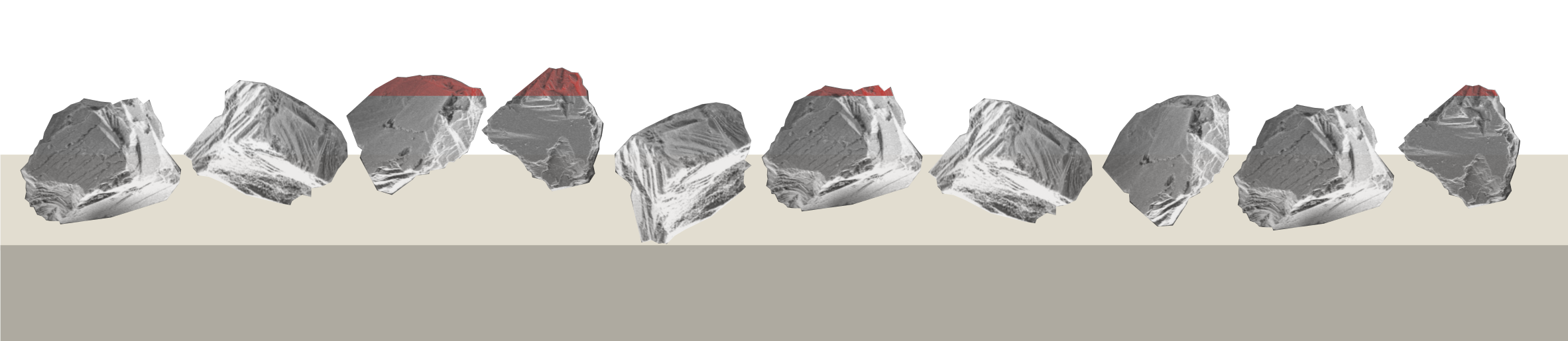
    In literature, this is called the difference between statistical edges (e.g., all you see above in the picture), and kinematically active edges. In order to clear up this point, take a look at the following diagram. It shows a typical grain distribution in a galvanic stone – actually, a pretty good one already. 90% of the grains are within 10% of their diameter variation. If you plot a straight line through these, you will see that only 4 out of the 10 grains are actually cutting into this imaginary straight line. I’ve coloured them red at their intersection. I like the colour red. It’s a professional thing.

    Illustration of a decent height distribution of similar grains in a galvanic binder. A portion of the grains above a certain horizontal line is coloured red, to show how few grains are typically active in the cutting process.

    Now, if we have a moving edge, the situation becomes a bit more complex. Because now, we don’t have a level, horizontal line of engagement. That would be the case of you lay your stone on top of a plate of steel, and becomes kinematically much more like lapping, with different material removal processes. Instead, what we have is a flat piece of metal (the knife edge), being dragged along the stone, and either by gravity or your hands being pushed into the material. If we imagine for a moment, that friction, elastic deformation & rebound are nonexistent, we can imagine that every grain basically removes the material to it’s very topmost, highest apex. But because the blade is moving, the “drag” behind it is finite, and a new portion of the blade is pressed into the grains and again thusly removed. I’ve illustrated this below. Please note that obviously, this is a very small section of the blade, and I’m not suggesting you should in any way be sharpening to a single sided edge.

    Illustration of the removed material from the 4 kinematic active edges. The blade movement and force vector are resembled by the black arrow.

    Now, here’s a couple of things we can deduce from this: the first is, the amount of grains that are cutting metal is actually pretty low. Secondly, because of the complex movement, the grains create some kinematic roughness in the blade. Our surface is not created by the highest grain, but by several of those, leaving a “ragged” surface behind. Nevertheless, the last grain leaves a track on the surface. With some use, these grains will wear first. In the space between grains, we will accumulate debris and swarf:

    SEM micrograph of a used TSPROF Blitz F1000. Some flattened grains and swarf stuck to the galvanic bond are visible. Instrument: Zeiss GeminiSEM560.

    Now, what does a very used galvanic stone looks like? For your viewing pleasure, and in the pursuit of the adventure of sharpness, I’ve sharpened edge after edge until my arms were sore and the stone was removing basically nothing:

    SEM micrographs of a very used TSPROF Blitz F1000. This one pretty much didn’t remove any material at all, any longer. Instrument: Zeiss GeminiSEM560.

    If we focus on one of the really flat grains, we can see how much is worn away, and how much swarf is embedded deeply into the galvanic bond:

    SEM micrograph of a VERY used TSPROF Blitz F1000. Instrument: Zeiss GeminiSEM560.

    Take a look at the grain directly above the red Kern logo (lovely, ain’t it?): This is pretty much completely rubbed flat, and level & even with the surrounding bond.

    If we flatten the grains in our previous illustrations, and apply the same GEDANKENEXPERIMENT of a blade being dragged along it, it looks like this:

    Illustration on how flattened grains are interacting with the material. For this, a horizontal line was drawn, but the removal of the material “simulated” via linear interpolation between the highest peak of a grain and the lowest portion of the next grain (kinematic distance between active grains).

    Now, a good question here would be to ask: Dr. Marv, why did you draw the engagements of these grains so shallow? They were taking much deeper cuts beforehand!

    For this, we will apply critical first principle thinking. When you sharpen, what you are doing is WORK. And I mean this in the physics sense of the word. Now, we will postulate that you know what you are doing, so you are not pushing unevenly. Whether the stone is worn or not, you apply the same force and speed to it, thus the same work. The work we are doing while grinding consists of several components: friction (which generates heat), plastic deformation (which removes material, generates heat), elastic deformation (“bounce back”) and shearing action. If you have a good lubricated stone (for example, with oil), and are moving slowly, friction and heat are not that big of an issue*. Elastic deformation is generally only a fraction of what is happening here. So, we could equal the work being done to material removal. If instead of only a few grains, all of which are taking a larger cross section out of the material, if you have more active grains, these will all have a similar cross section (maybe a bit larger, as we are moving towards their center and therefore maximum diameter), your actual depth of cut will diminish.

    *authors note: total lie here. Friction ALWAYS is a super big issue, and actually becomes worse, the duller your grain is. But for our Gedankenexperiment, it doesn’t change a lot. Just makes it less dramatic than my drawing. Trust me. I’m a doctor and I draw pretty illustrations. Also, I have stuff to prove this.

    The following illustration is showing the new, much smaller intersection from the beforehand drawn kinematic active grains.

    Illustration, highlighting the kinematic active grains and their active cross section in red. To see how much the grains are worn down, their full shape is visible with low opacity.

    Now, what is the result of this? To prove my point, the above theory and showcase this, I’ve prepared two edges. One, with a brand new Blitz F1000. One, with the very much destroyed one. The steel used is M398 at 63.5 HRC, the edge was prepared with progressively finer galvanic stones (150-220-400-800) at 17 DPS.

    Let’s compare the result from an optical perspective:

    Optical micrograph of the same edge prepartion with two different usage states. Left side: brand new galvanic stone, right side: very used up galvanic stone. Instrument: iPhone 15 Pro with a 120x macro loupe, hence the distorted picture on the right.

    This is a pretty drastic difference, the blade on the right side is much smoother, shinier, even glossy. It looks like a finer stone made this! …wait, what?

    Luckily, I have access to better microscopes than my phone. Let’s compare what these two edges look like in the scanning electron microscope:

    SEM micrographs of a sharpened blade, 250x magnification (FOV: 505µm). First/left picture: new stone, right/second picture: used stone. Instrument: Thermo Fischer PhenomXL.

    SEM micrographs of a sharpened blade, 500x magnification (FOV: 505µm). First/left picture: new stone, right/second picture: used stone. Instrument: Thermo Fischer PhenomXL.

    Now, this is a stark difference. The new stone created a sharp, uneven morphology. Lot’s of micro prows, deeper scratches and general uneven surfaces are visible. The used up stone created a much smoother surface. There are some scratches, especially closer to the edge. The surface further from the apex is very smooth and rounded, giving it a burnished appearance.

    SEM micrographs of a sharpened blade, 1000x magnification (FOV: 505µm). First/left picture: new stone, right/second picture: used stone. Instrument: Thermo Fischer PhenomXL.

    At higher magnification, we can make out a sharper apex from the new stone, but also more debris, burr and carbide cracking. The apex from the used stones looks more rounded and dull.

    Now, while the SEM is a tool that is fantastic in spotting small details, it’s spatial (in the direction of the beam) resolution isn’t super good. To further analyse what we are seeing, I’ve used our Bruker Alicona µCMM to record some 3D data of the blade apex. It’s a very expensive, optical coordinate measurement machine that uses the measurement principle of focus variation to record height data over a surface area. Why did I use that one and not the Zygo interferometer? Well, the lovely zygo is currently at an exhibition, so I had to make do with what we had *crys in millions of metrology equipment*.

    3D height maps of the two measured edges. Left/first picture: new stone. Right / second picture: Used stone. Instrument: Bruker Alicona µCMM, 50X objective lens, singe FOV high resolution focus variation scan. Data is leveled and outliers removed (0.25%)

    Now, one thing is immediately visible: The new stone created a very flat surface, with deeper, and very direction scratches. The used stone created a slightly rounded of (convex) surface, with smoother roughness. The scratches are directional, but there are some deeper ones at a steeper angle.

    With this height data, we can start doing real analysis. First, let’s take a look at the width and depth of the scratches. For this, I’ve filtered the micro roughness via a gaussian filter with a cutoff of 0.8 micrometre:

    New galvanic stone blade: Above: filtered surface to remove micro roughness and make step height determination easier. Below: Step height determination. Software used: Digital Surface Mountains Map. <3

    and extracted a profile perpendicular through the scratch: Step analysis shows a width of 11 µm, with a maximum “height” (or depth) of 1 µm.

    Comparing this to the used stone, with identical workflow (filtering, extraction of profile, step height determination):

    Used galvanic stone blade: Above: filtered surface to remove micro roughness and make step height determination easier. Below: Step height determination. Software used: Digital Surface Mountains Map. <3

    We arrive at a similar width (10.5 µm), but a much lower maximum height (depth) of 0.38 µm. So, without question we can answer a lemma put up at the beginning of this post: galvanic bound grinding stones do not become finer over time. But because the grains flatten out, their actual depth of cut and the grooves they are creating are more shallow and smoother.

    Let’s take a look at the surface metrology data we can extract. For this, I’ve extracted an area of the scan, leaving out the very fine apex of the blade, as we have some measurement artefacts on this one (“batwings”, basically diffraction light at a sharp and burry edge). For those of you working in the manufacturing world, feast your eyes on the ISO 25178 parameter table. This is how you state roughness: clear identification of the workflow, filters and parameter settings used, together with a coloured heat map of the surface recorded.

    Surface heatmap and ISO 25178 roughness (S-L) parameters of the edge ground with the new TSPROF Blitz F1000 stone.

    Now, what can we extract from this? The quadratic surface roughness Sq is a super fine parameter to evaluate surface roughness, as it is also the “power” of a surface, and therefore directly proportional to how shiny you experience this. We’ve achieved a value of 0.28 µm here, which is about what I would expect from this grit of galvanic stone. The kurtosis (Sku) is around 3, which is where “sharper” profiles start. This means the surface is more of a zig-zag instead of a well rounded sine profile.

    We have a low material ratio Smr (17%), so that means only a fraction of our surface is found at the top 1 µm of our height data. If this was a bearing surface (and during a cut it is!) it would have very few spots it would actually have contact with. The auto-correlation length Sal is the dominant spatial structure – here we can see that the fine scratches we see at a direction of 144° to the x-axis of our recording (compare parameter Std, texture direction) are spaced at 1.35 µm.

    Surface heatmap and ISO 25178 roughness (S-L) parameters of the edge ground with the used TSPROF Blitz F1000 stone.

    Comparing the used surface with the one above, we can see a significant improvement of the surface roughness Sq at 0.22 µm (27% lower), a much higher kurtosis (Sku, 4.45 µm). The material ratio Smr is also crazy high – 79% definitely point towards a “flattened”, e.g. burnished surface. The auto correlation length Sal didn’t really change, as did the texture direction (153° compared to 144°).

    So, that’s it folks. I think this shows that galvanic stones do not become “finer” over time. Surface finish improves, as the grains are flattened, outlier grains are torn out or shattered, and a burnishing process begins. The shape of the blade seems to deteriorate – at least with my skill of sharpening and on a TSPROF K03.

  • A brief study on sharpening stones – Part 6 – Edge Pro Matrix Stone 4000 Grit (5 micron diamond, resin)

    This is part of a series of blog posts – looking into the appearance and composition of commercially available sharpening stones. If you are interested in the previous episodes:

    Part 1 is about the Fällkniven DC3 , Part 2 is about the DMT mini W7C, Part 3 is about the TSPROF Blitz F1000, Part 4 is about a natural jade stone, Part 5 is about the Venev 5/3 Diamond Resin Stone.

    If you have some suggestion on what I should look at next, or want to share your super secret DIY stones, I could be persuaded to open the bag of analytical devices… hit me up on Instagram under @marvgro for that.

    Today’s sharpening stone is the Edge Pro Matrix Stone at 4000 grit, which according to the manufacturer equals 5 micrometre grain size. It’s their stone “made for modern super steel” and apparently self sharpening by loosening grains over time. 🙂

    It’s a super smooth, very fine stone. Stroking it with your finger, it just feels barely sticky, while scratching it with your fingernail shows some resistance – but can also leave a small groove.

    Optical micrographs of the Edge Pro Matrix Stone (4000). The scale bar is visible in the lower right corner. Instrument: Leica Emspira.

    The microscope supports this picture. A very uniform, smooth surface. The corners around the stone are slightly beveled. At higher magnifications, grains start to become visible. Do we have a new king of agglomeration here? Let’s throw it into the SEM to check it out.

    The first thing I saw in the SEM was…nothing. Because this stone is so smooth, and also because they really seem to use no fillers, additives or anything else, it immediately starts charging like crazy. The resin they are using is also covering the topmost layer, making it hard to distinguish between resin and diamond. Well, this ain’t a BEAST of a scanning electron microscope for nothing. We’ve equipped it with multiple sensors and it is a very versatile device. To make an image visible, I’ve bumped up the accelerating voltage. To explain why this is different to the other pictures you’ve seen in this blog before, I think I need to detour for a small moment.

    In a scanning electron microscope, the image is created by using a beam of electrons, and moving that one in regular lines across the surface of a sample. At every point it hits the sample, interaction happens. This interaction is typically either an elastic reflection of the incident electrons (back scattered electrons, BSE), or the ejection of electrons from a shell around the atoms (secondary electrons, SE). The BSE are showing you mostly elemental contrast, whereas the SE show you a topographical (surface) contrast. Nevertheless, with good enough sensors, both show you a bit of the information of the other type. Now, the BSD (back scatter detector) is pretty robust, and works nicely at lower vacuum. Because the sample is non conductive, it will experience static charge. Lowering the chamber vacuum introduces moisture (H2O) into the chamber, and this is enough to reduce the static charge on the sample. Unfortunately, lower vacuum also means lower resolution, and the BSD doesn’t give us great surface morphology to begin with. A workable way to combat this is to increase the accelerating voltage. This will not only give you more signal, reduce noise, but also increase the interaction volume of the beam. Basically, you are now looking a couple micrometre deep into the material!

    SEM Micrographs of the Edge Pro Matrix Stone (4000). Note that these pictures are BSD and at high accelerating voltage. Instrument: Zeiss GeminiSEM560.

    We can see that this stone really only contains a matrix and the diamond grit. All grains are small with tight controlled size distribution. No fillers or other abrasives are visible. The matrix is relatively dense, and the atomic contrast of it is similar to the diamond next to it. This is the first stone I’ve looked at that contains no fillers. Unfortunately, with this comes two problems: Quite a bit of agglomeration is visible, with often 3 or more grains sticking close to each other. The second is the retention of the grains – we can see on this unused stone already, that nearly no grain is sticking out of the surface. Even the manufacturers dressing process removed the majority of all surface grains. I would expect this stone to be quite slow and soft. Because of the simple composition, no EDS was recorded.

    The surface under the white light interferometer shows a smooth, regular and low roughness surface.

    White light interferometry height map of the Edge Pro Matrix Stone (4000). Instrument: Zygo Nexview NX2, Objective Lens: 10X. Stitched overview of 4×4 images.

    The overall height distribution is lower than for example on the similar grit Venev stone. The actual contact surface, at least brand new, should be relatively low, as it doesn’t show a lot of plateaus in the height map.

    ISO 25178 parameters of the Matrix Pro Stone (4000).

    The areal surface parameter support this observation. This is one very smooth stone, with very low roughness and material ratio.

    In order to evaluate the sharpening performance of these stones, 3 blades were sharpened. In order to evaluate the sharpening performance of this stone, a blade was sharpened with it. I am using a standardised testing procedure, read about it here. Nevertheless, it’s 65 HRC M398, and sharpened to 17 DPS with resin bond diamond stones down to 10 µm. Afterwards, the tested stone is used, first in a back and forth movement until the surface becomes homogenous, and then alternating, edge trailing strokes (5-5-3-2) on each side, for a total of 20 strokes per side. No pressure is applied but the weight of the apparatus. Then the Pro Matrix stone comes into play.

    SEM micrographs of the sharpened blade. Note that the last picture (2kx magnification) isn’t a center zoom of the one before, but slightly to the left of the FOV, as I identified some carbide cracking that I wanted to visualise in higher detail. Instrument: Thermo Fischer PhenomXL Scanning Electron Microscope.

    The surface of the edge is much smoother than with the equally sized Venev sharpening stone. The edge shows a low waviness and no identifiable burr. This is certainly a statement to the heat treat of the steel (made by Roman Kasé!), but also to the stone. Some deeper grooves are visible, which could be because of the agglomeration, or a rolling grain that got loose. The low material removal rate gives a high cutting pressure, likely leading to the carbide cracking and edge breakouts at carbide-steel interfaces. This is a cool stone, with a nice feeling while sharpening, awesome result and very finely made. I like it. If only it was a faster stone!