Tag: sharpness

  • A brief study on sharpening stones – Part 6 – Edge Pro Matrix Stone 4000 Grit (5 micron diamond, resin)

    This is part of a series of blog posts – looking into the appearance and composition of commercially available sharpening stones. If you are interested in the previous episodes:

    Part 1 is about the Fällkniven DC3 , Part 2 is about the DMT mini W7C, Part 3 is about the TSPROF Blitz F1000, Part 4 is about a natural jade stone, Part 5 is about the Venev 5/3 Diamond Resin Stone.

    If you have some suggestion on what I should look at next, or want to share your super secret DIY stones, I could be persuaded to open the bag of analytical devices… hit me up on Instagram under @marvgro for that.

    Today’s sharpening stone is the Edge Pro Matrix Stone at 4000 grit, which according to the manufacturer equals 5 micrometre grain size. It’s their stone “made for modern super steel” and apparently self sharpening by loosening grains over time. 🙂

    It’s a super smooth, very fine stone. Stroking it with your finger, it just feels barely sticky, while scratching it with your fingernail shows some resistance – but can also leave a small groove.

    Optical micrographs of the Edge Pro Matrix Stone (4000). The scale bar is visible in the lower right corner. Instrument: Leica Emspira.

    The microscope supports this picture. A very uniform, smooth surface. The corners around the stone are slightly beveled. At higher magnifications, grains start to become visible. Do we have a new king of agglomeration here? Let’s throw it into the SEM to check it out.

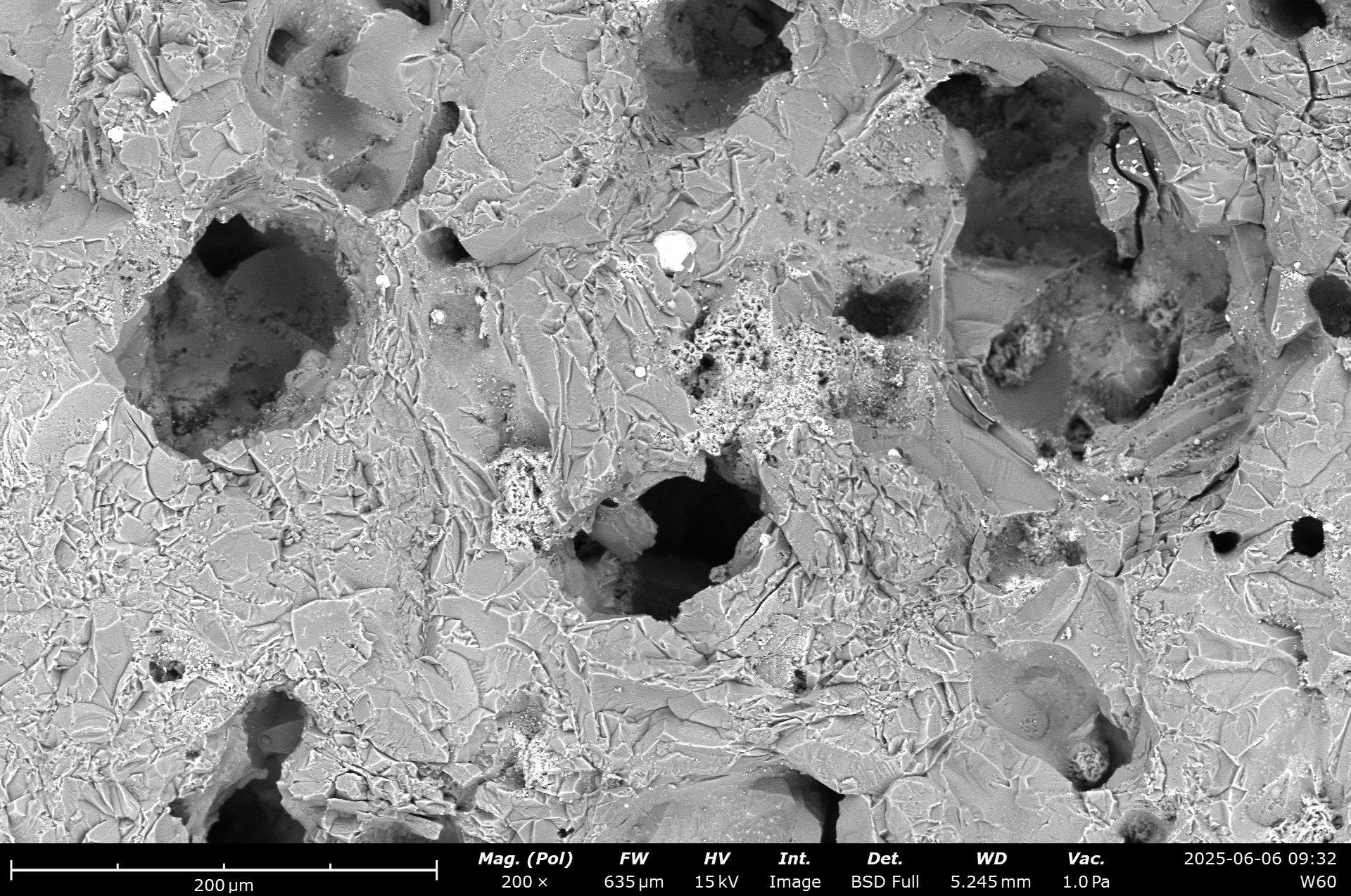
    The first thing I saw in the SEM was…nothing. Because this stone is so smooth, and also because they really seem to use no fillers, additives or anything else, it immediately starts charging like crazy. The resin they are using is also covering the topmost layer, making it hard to distinguish between resin and diamond. Well, this ain’t a BEAST of a scanning electron microscope for nothing. We’ve equipped it with multiple sensors and it is a very versatile device. To make an image visible, I’ve bumped up the accelerating voltage. To explain why this is different to the other pictures you’ve seen in this blog before, I think I need to detour for a small moment.

    In a scanning electron microscope, the image is created by using a beam of electrons, and moving that one in regular lines across the surface of a sample. At every point it hits the sample, interaction happens. This interaction is typically either an elastic reflection of the incident electrons (back scattered electrons, BSE), or the ejection of electrons from a shell around the atoms (secondary electrons, SE). The BSE are showing you mostly elemental contrast, whereas the SE show you a topographical (surface) contrast. Nevertheless, with good enough sensors, both show you a bit of the information of the other type. Now, the BSD (back scatter detector) is pretty robust, and works nicely at lower vacuum. Because the sample is non conductive, it will experience static charge. Lowering the chamber vacuum introduces moisture (H2O) into the chamber, and this is enough to reduce the static charge on the sample. Unfortunately, lower vacuum also means lower resolution, and the BSD doesn’t give us great surface morphology to begin with. A workable way to combat this is to increase the accelerating voltage. This will not only give you more signal, reduce noise, but also increase the interaction volume of the beam. Basically, you are now looking a couple micrometre deep into the material!

    SEM Micrographs of the Edge Pro Matrix Stone (4000). Note that these pictures are BSD and at high accelerating voltage. Instrument: Zeiss GeminiSEM560.

    We can see that this stone really only contains a matrix and the diamond grit. All grains are small with tight controlled size distribution. No fillers or other abrasives are visible. The matrix is relatively dense, and the atomic contrast of it is similar to the diamond next to it. This is the first stone I’ve looked at that contains no fillers. Unfortunately, with this comes two problems: Quite a bit of agglomeration is visible, with often 3 or more grains sticking close to each other. The second is the retention of the grains – we can see on this unused stone already, that nearly no grain is sticking out of the surface. Even the manufacturers dressing process removed the majority of all surface grains. I would expect this stone to be quite slow and soft. Because of the simple composition, no EDS was recorded.

    The surface under the white light interferometer shows a smooth, regular and low roughness surface.

    White light interferometry height map of the Edge Pro Matrix Stone (4000). Instrument: Zygo Nexview NX2, Objective Lens: 10X. Stitched overview of 4×4 images.

    The overall height distribution is lower than for example on the similar grit Venev stone. The actual contact surface, at least brand new, should be relatively low, as it doesn’t show a lot of plateaus in the height map.

    ISO 25178 parameters of the Matrix Pro Stone (4000).

    The areal surface parameter support this observation. This is one very smooth stone, with very low roughness and material ratio.

    In order to evaluate the sharpening performance of these stones, 3 blades were sharpened. In order to evaluate the sharpening performance of this stone, a blade was sharpened with it. I am using a standardised testing procedure, read about it here. Nevertheless, it’s 65 HRC M398, and sharpened to 17 DPS with resin bond diamond stones down to 10 µm. Afterwards, the tested stone is used, first in a back and forth movement until the surface becomes homogenous, and then alternating, edge trailing strokes (5-5-3-2) on each side, for a total of 20 strokes per side. No pressure is applied but the weight of the apparatus. Then the Pro Matrix stone comes into play.

    SEM micrographs of the sharpened blade. Note that the last picture (2kx magnification) isn’t a center zoom of the one before, but slightly to the left of the FOV, as I identified some carbide cracking that I wanted to visualise in higher detail. Instrument: Thermo Fischer PhenomXL Scanning Electron Microscope.

    The surface of the edge is much smoother than with the equally sized Venev sharpening stone. The edge shows a low waviness and no identifiable burr. This is certainly a statement to the heat treat of the steel (made by Roman Kasé!), but also to the stone. Some deeper grooves are visible, which could be because of the agglomeration, or a rolling grain that got loose. The low material removal rate gives a high cutting pressure, likely leading to the carbide cracking and edge breakouts at carbide-steel interfaces. This is a cool stone, with a nice feeling while sharpening, awesome result and very finely made. I like it. If only it was a faster stone!

  • A brief study on sharpening stones – Part 1 – Fällkniven DC3

    The absurd amount on sharpening stones on the market should ring some alarm bells. The first is: there must be a lot of money in this. The second: what’s the difference between them? The third: which is the ideal one (for me)?

    I’ve ordered and then analysed a couple of different grinding stones. This is probably going to become an ongoing series of blog posts, whenever I get new and exciting grinding stones. If you have some suggestion on what I should look at next, or want to share your super secret DIY stones, I could be persuaded to open the bag of analytical devices… hit me up on Instagram under @marvgro for that.

    Fällkniven DC3 (diamond/ceramic whetstone)

    According to the manufacturer’s homepage, this is a “diamond grit 25 micron, sapphire ceramic grit 5 micron”. Let’s take a look!

    Optical Micrograph of the diamond side. Magnification and scale bar are visible on the lower right part of the image. Microscope: Leica Emspira

    The diamond side is coated in TiN. Typically, this coating can be found on cheaper HSS tooling, as it’s quite hard (2400-2700 HV), but also slick and doesn’t let chips adhere. It’s a curious choice to put on a grinding stone, as the grit used here (diamond) is quite a bit harder – depending on the grain orientation, it clocks in at 10000 HV. It’s certainly nice looking though, and I’d postulate that this is the main reason it is applied to any sharpening stone.

    SEM Micrographs of the Fällkniven DC3 stone. It shows quite a large range of grain sizes. Instrument: Thermo Fischer PhenomXL Scanning Electron Microscope

    SEM pictures show gritty, sharp diamonds. The range distribution of the visible grains (measured at their largest diagonal distance) ranges from 50 to 75 micrometre, with a strong weighting towards the upper end. The grit’s have a distinct checkered look to them – this is the coating, sticking to some parts of the diamond, and not adhering to others. It is very likely that the first use of the stone would remove the coating at any point that is in contact with a blade.

    Energy dispersive x-ray spectroscopy (EDS) inside the scanning electron microscope show the coating (Ti, N), the diamond grain (C) as well as the galvanic binder around the grains (Ni). Instrument: Thermo Fischer PhenomXL Scanning Electron Microscope

    In order to faciliate a better sense of depth and size, a surface scan was undertaken via white light interferometry. This creates a very high resolution height map – the Z resolution here is absurdly small, where’s the X/Y resolution (“spatial resolution”) follows the Abbe diffraction limited law.

    White light interferometry height map of the diamond surface. Instrument used: Zygo Nexview NX2, Objective Lens: 10X. Stitched overview of 4×4 images.

    We can see the typical galvanic bound height distribution – unevenly spaced grains with some very high outliers. This is the main reason that galvanic stones leave larger scratches and commonly a worse surface than a similar grain sized vitrified or resin bound stone.

    ISO 25178 surface parameters of the Fällknives DC3 diamond side.

    The ISO25178 parameters show a rough surface (Sa/Sq are the arithmetic respective quadratic surface roughness). Sz is the total height of the surface. Very indicative of the distribution is the parameter “Sdc”, which shows the range between the lowest 10% and highest 90% of the measured points. This is a good indicator how “even” the height distribution is. A perfect flat surface would have a value of 0 here, whereas a widely spread surface shows a wider range. It’s a usefull parameter to compare stones, but leaves out the 10% outliers at every end. Sku, the kurtosis shows how “sharp” the surface data is. Typically, a value below 3 is considered flat, whereas values above 3 are considered very sharp.

    The other “ceramic” side shows a typical ceramic abrasive mix.

    SEM images show a pretty uniform, surface with some large voids.

    SEM micrographs of the surface morphology. A typical, sintered alumina oxide appearance with some foreign particles (darker colour in the BSD image) and large voids are visible. Instrument: Thermo Fischer PhenomXL Scanning Electron Microscope

    While the void size is suprising, this certainly allows for some swarf build-up. 🙂 Some metal particles (bright white colour), but also some different abrasive grains (slightly darker grains) are visible. The detector used is a back-scatter detector. Here, besides the topographical contrast, one also has a contrast based on the weight of the element. The rule of thumb here is: the heavier the element, the brighter the returned pixel is. Pure metals are typically the brightest, whereas ceramics or diamonds are of darker colour.

    EDS analysis of the chemical composition. The colour corresponds to the individual element, visible above the scale bar. Instrument: Thermo Fischer PhenomXL Scanning Electron Microscope

    Chemical analysis show several large SiC grains, as well as Al2O3 grains. As sapphire is chemically Al2O3, just in a monocrystalline configuration, I think we have identified plenty about the compoistsion. Trace elements of metals and Calciumoxide (blue colours) are likely impurities from manufacturing.

    White light interferometry height map of the ceramic surface. Instrument used: Zygo Nexview NX2, Objective Lens: 10X. Stitched overview of 4×4 images.

    The whitelight interferometry surface map shows a relatively rough surface. large voids are visible, the range of height values doubles compared to the diamond size. On the other hand, the uppermost part of the surface shows a higher plateau region. The contact area likely is higher on this stone side. Sku, the kurtosis shows how “sharp” the surface data is. Typically, a value below 3 is considered flat, whereas values above 3 are considered very sharp. Here, a much lower value than on the diamond surface can be seen.

    Combined with the low sharpness of the dull ceramics, a burnishing effect is expected, improving the appearance of a blade with very low effort.

    ISO 25178 surface parameters of the Fällknives DC3 ceramic side.

  • Comparison of commercial wheels on a Tormek T8

    Comparison of commercial wheels on a Tormek T8

    I’ve started my journey into “knife sharpening” a couple of years back with some cheap, free hand (unguided!) waterstones from a large, american online delivery service. I think it goes without saying, that my experience with those was more than frustrating. Messy, frustrating and kind of disappointing in terms of achievable finish and sharpness. Probably caused by 2 things: my lacking skills, and the poor quality of those. Improvements were made with a higher quality stone, and finally some galvanic bound diamond sharpening stone. Nevertheless, I was longing for something powered. After all, if it’s not driven by an electric motor, how good can it be?

    My good friend Roman, the steel-virtuoso from Switzerland (check out: https://www.kase-knives.com/ or find him on http://instagram.com/kknives_switzerland ) convinced me that the only real way to go is the Tormek T8. It’s a rotary grinding machine, where you clamp your knife in a (hopefully) symmetric holder and then grind along a bar. By setting the height of the bar, you can adjust the angle of the knife blade.

    My Tormek T8, on the day it was delivered in December 2024.

    Now, if you just want a sharp knife, in a decent amount of time, and don’t have two left thumbs, this is a fantastic machine. But: it’s not the end. And with this, I dug deep down into the rabbit hole that is sharpening.

    The original wheel is a galvanic bound diamond wheel. What does this mean? It uses an abrasive (in this case, diamond!), and this abrasive is fixed as a single layer to a metal body. The bond holding the diamond on the wheel is typically electroplated nickel. Under the scanning electron microscope, such galvanic bonds look like this:

    Here, the diamond grit is visible as black, little grains. The metal bond is the smooth, light coloured matrix around them. On the lower left o every picture, you can see the scale bar. For a better impression of the size, “FW” is the field of view, so the width of the image from left to right. These images were taken with a small, capable desktop SEM (a Thermo Fischer PhenomXL, which has a thermionic electron source and a 100x100x40 mm large sample chamber). The height map was also created via selectively switching the 4 sectors of the BSD sensor inside the SEM.

    The advantages of galvanic bound grinding bodies are plenty: They are very clearly defined in their shape, the bond is very strong (it is difficult to tear out a grain, so grain retention is high), and they are considered “easy cutting”, because the large gap and overhang of the grinding grains lower grinding pressure and have plenty of space for removed material (the “swarf”).

    The downside is: you only have 1 layer. Once that is gone, your grinding wheel is used up. It’s difficult to embed very small grains. And sometimes, a grain sticks out really far – this leaves a long streak on your surface, digging really deep. And then the internet believes, you can’t dress them…

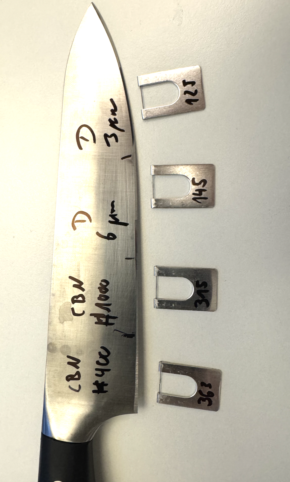
    At this point, I decided to go down the rabbit hole and get a couple of wheels that are considered “high end”. Mainly, a #400 Grit CBN wheel, a #1000 grit CBN wheel (both galvanic bond), and a 6 micrometre and 3 micrometre diamond wheel (both resin bond). And while they make a very pretty and glossy surface, and a sharp knife edge, I was curious to dig a little deeper into how the surface looks like.

    For this, I prepared a knife with increasingly finer edge preparation. First, only the #400 grit CBN wheel, then a section of the blade with #400 and then #1000; followed by a section going through the two CBN wheels and then the 6 micrometre diamond wheel, and then at the very tip, all wheels down to the 3 micrometre diamond wheel. The knife used was a cheap “IKEA” knife from stainless steel. I choose 19 degrees per side (DPS). You’ll see in a moment why I choose a cheap knife.

    The following gallery shows optical microscopy micrographs of the cutting edge quality:

    Optical microscopy shots of the cutting edge prepared with #400, #100 grit CBN, as well as (darker colored, smoother) 6 micrometre and 3 micrometre (nearly “flawless” at this magnification) diamond resin wheels.

    I then cut the blade apart, and analysed the cutting edge quality in the SEM.

    The cutting edge after the #400 grit CBN wheel. SEM micrographs show an overview, the surface morphology in the middle of the cutting chamfer as well as a detail view of the cutting apex.

    This piece of the blade measured in at 363 bess. The resulting BESS media looked pretty torn up:

    The #1000 grit CBN wheel, which is often considered the “finest” sensible CBN wheel, left a much nicer finish:

    The cutting edge after the #1000 grit CBN wheel. SEM micrographs show an overview, the surface morphology in the middle of the cutting chamfer as well as a detail view of the cutting apex.

    The BESS measured in at 315, and the media looks much smoother cut:

    With the 6 micrometre diamond wheel, the finish is starting to approach the resolution limit of this small desktop SEM, as it becomes smooth enough to be nearly flat.

    The cutting edge after the 6 micrometre diamond resin wheel. SEM micrographs show an overview, the surface morphology in the middle of the cutting chamfer as well as a detail view of the cutting apex. Note the two additional images at a higher magnification to showcase the burr formation.

    The BESS value clocked in at a respectable 145. The media is nicely sliced:

    The final “polish” was done with the 3 micrometre diamond resin wheel. This one already exhibits quite a bit of pressure, and doesn’t remove a lot of material.

    The cutting edge after the 3 micrometre diamond resin wheel. SEM micrographs show an overview, the surface morphology in the middle of the cutting chamfer as well as a detail view of the cutting apex. Note the two additional images at a higher magnification to showcase the burr formation.

    The BESS score clocked in at 125. The media is properly cut: